images are taken from: http://www.smashingmagazine.com/2008/08/24/45-beautiful-motion-blur-photos/
Motion blur is often caused by the long exposure time of the camera. Exposure time is the duration of time that the camera's shutter is open. In this case, the object moved within the exposure time causing the blur in the image captured.
For activity, we restored motion blurred images. In doing this we used degradation modeling. to be able to blur a given image. Here, we consider the case where in the image represented by f(x,y) has been blurred by the linear movement between the object and the image acquisition device used. Assuming that the opening and closing of the shutter happens instantaneously, the blurred image is given by
 Equation 1
where xo and yo represents the time varying components of motion in the x and y directions, and T represents the exposure time.
Consequently, the Fourier transform of the bulrred image is given by,
 Equation 2
where G(u,v) and F(u,v) blurred and original images in frequency space while H(u,v) is the degradation function in Fourier space given in the following equation.
 Equation 3
where a and b are the total distances for which the image has been displaced both in the x and y directions.
After blurring the image, gaussian noise was also added into it. Thus G(u,v) can now be expressed as
 Equation 4
where N(u,v) is the added noise in frequency space.
Now to be able to recover the original image from its blurred counterpart we used the Minimum mean square error or Weiner filtering. In this method, the image and the noise added are considered as random processes. The orginal image in frequency space is then given by,

Equation 5
Where Sn and Sf are the power spectrum of the noise and the original image both in frequency space. However, in reality the power spectrum of the ungraded or the original image is unknown. Thus the equation for the restored image can be written as,
 Equation 6
where K is a constant.
Using Equations 2 and 3, blurred image of the text below with a and b equal to 0.1 and T = 1 were simulated. This blurred image was then used to recover the original image using equations 5 and 6. These images are shown below.
 Original image

Using equation 6, the original image was recovered for varying values of K. What I used here are: 5, 3, 0.01 and 0.00001.

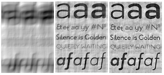
As can be seen from the figure above as K decreses, the recovered image looks more like the original. The values of a and b (x and y displacements) were also varied. The recovered images are shown below. The First column of the suceeding 4 sets of images are the blurred images, the second column are the recovered images using Equation 6 and the third column are the recovered images using Equation 5.
 a & b = 0.9

 T = 3
T = 3
 T = 5
T = 5
References:
[1] Activity 19: Retoration of Blurred Images Manual
For activity, we restored motion blurred images. In doing this we used degradation modeling. to be able to blur a given image. Here, we consider the case where in the image represented by f(x,y) has been blurred by the linear movement between the object and the image acquisition device used. Assuming that the opening and closing of the shutter happens instantaneously, the blurred image is given by
 Equation 1
Consequently, the Fourier transform of the bulrred image is given by,
 Equation 2
 Equation 3
After blurring the image, gaussian noise was also added into it. Thus G(u,v) can now be expressed as
 Equation 4
Now to be able to recover the original image from its blurred counterpart we used the Minimum mean square error or Weiner filtering. In this method, the image and the noise added are considered as random processes. The orginal image in frequency space is then given by,

Equation 5
 Equation 6
Using Equations 2 and 3, blurred image of the text below with a and b equal to 0.1 and T = 1 were simulated. This blurred image was then used to recover the original image using equations 5 and 6. These images are shown below.
 Original image

Using equation 6, the original image was recovered for varying values of K. What I used here are: 5, 3, 0.01 and 0.00001.

As can be seen from the figure above as K decreses, the recovered image looks more like the original. The values of a and b (x and y displacements) were also varied. The recovered images are shown below. The First column of the suceeding 4 sets of images are the blurred images, the second column are the recovered images using Equation 6 and the third column are the recovered images using Equation 5.
 a & b = 0.9

a & b = 0.9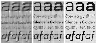 a & b = 0.01
 a & b = 0.001
 T = 0.001
 T = 0.01
 a & b = 0.01
 a & b = 0.001
As can be observed in the images above, as the value of a and b decreases the recovered images looks more like the original image. This can be seen especially in the last set of images where a and b are equal to 0.001. This behaviour is expected since a and b are the displacements of the object in the x and y directions. Small values of a and b only mean that the object moved a small distance from its original position while its image is being captured. Thus as the value of a and b increases the generated blurred image becomes more blurred.
The values of the exposure time, T, was also varied. The recovered images are shown below. The First column of the suceeding 4 sets of images are the blurred images, the second column are the recovered images using Equation 6 and the third column are the recovered images using Equation 5.
The values of the exposure time, T, was also varied. The recovered images are shown below. The First column of the suceeding 4 sets of images are the blurred images, the second column are the recovered images using Equation 6 and the third column are the recovered images using Equation 5.
 T = 0.001
 T = 0.01
 T = 3
T = 3
 T = 5
T = 5
As can be observed from the four sets of images above, as the value of T increases, the recovered images look more like the original one. Also, observe that the generated blurred images for small value of T are dark. If we will recall the definition of T, it is the duration of the exposure time or the duration of time that the shutter of the imaging device is opened. For small values of T, small amount of light will be able to enter the imaging system. Thus, the generated dark blurred images.
A possible extension of this activity is the recovery of the "unblurred" image of a nactual blurred image taken. However to be able to do this, one must have the knowledge of the degradation function of the blurred image.
For this activity I thank Irene Crisologo, Thirdy Buno, Jaya Combinido and Miguel Sison for the helpful discussions.
I give myself a grade of 10 for I was able to do all the required tasks for this activity.
References:
[1] Activity 19: Retoration of Blurred Images Manual